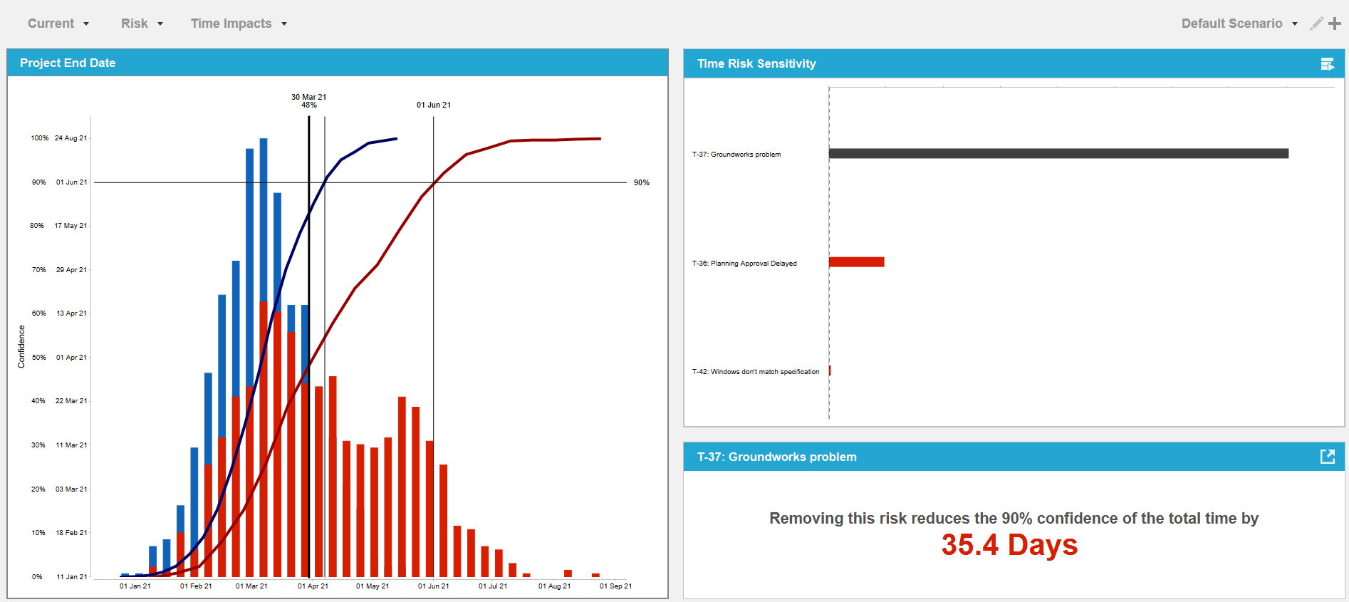
Monte Carlo simulation uses repeated random sampling to calculate results about physical and mathematical systems. It uses uncertainty in its inputs to generate a range of possible outcomes, which are then reported as results with a degree of mathematical confidence. The method tends to be used when it is infeasible or impossible to compute an exact result with a deterministic algorithm.
Describing Uncertainty and risk events

The uncertainty used as inputs to Monte Carlo simulation is described using probability distributions, which define the range of values a variable might take, and the likelihood of those values occurring.
The most commonly used probability distribution used for modelling project and business uncertainty is the Triangular distribution, so called because it is defined by three points – a minimum, likely and maximum value. For example, the time required to dig the foundations for a new house may be a minimum of 10 days (best case), likely of 12 days and maximum of 15 days (worst case). This is called a three point estimate and is often based on historic information and experience (a building firm that has built hundreds of houses over several years will have a pretty good idea).
 Monte Carlo simulation is also used to model project and business risk events. In this case, two probability distributions are required. First a Bernoulli distribution is used to model whether the risk event occurs – resulting in either a True or False result (e.g. a coin can be used to model a risk that has a 50% chance of occurring – heads it happens, tails it doesn’t). Second, the uncertain impact of the risk is described, typically using a Triangular distribution.
For example, while digging the foundations for your house, you may suffer from extremely bad weather, causing a delay before you can continue with your task. The probability of extremely bad weather (the event) might be 5% and your estimate of the impact (the uncertainty) might be between 2 and 8 days, but most likely 4.
Using Monte Carlo Simulation
Even in a small project or business model, you are likely to have hundreds of uncertain tasks and dozens of possible risk events. You need a mechanism for understanding what this means in terms of the possible outcome (success or failure). Taking a simplistic approach, you could calculate the worst case scenario, by adding the maximum values for all variables and assuming all of the risks happen. But this will produce a very pessimistic outcome, with the result that you will probably never embark on building your house. Similarly, taking the most optimistic view will give you a false picture of your ability to deliver on time and budget, resulting in substantial overrun and losses.
Monte Carlo simulation is used to create a picture of the outcomes between the optimistic and pessimistic scenarios, with the results tending to a bell shaped curve (a Normal distribution). The mathematical basis for this shape is the Central Limit Theorem, where the combination of a large number of independent random variables will converge to a Normal distribution. The only requirement is that you repeat the Monte Carlo ‘experiments’ enough times, to ensure a representative set of random samples have been used.
Understanding the results
The Monte Carlo set of outcomes (results distribution) can be interrogated to understand the confidence of meeting specified targets. For example, if you run the Monte Carlo simulation 1000 times, you will produce 1000 potential completion dates for your house. To work out the confidence of meeting a 30th July deadline, count up the number of results that lie to the right of that date. If there are 200 such results, then you know that there is a 20% chance (200/1000) that you will overrun. Conversely, you can be 80% confident that you will finish on time or early. The benefit of Monte Carlo, is that you can generate intermediary results in addition to the overall outcome, for example, you can calculate the confidence of meeting milestones as well as the project end date.

Further results can be gleaned from the Monte Carlo outputs. One very useful measure is sensitivity, which is often portrayed in a Tornado diagram. Sensitivity measures how much influence an input variable has on your outcome. For example, any risk event or uncertainty experienced while digging your foundations may have a very large influence on your project end date, whereas problems when you are painting the walls may not factor into the end date at all. The Tornado chart is particularly useful in highlighting which tasks in your project are the most likely cause of delay or overrun. This helps focus on which areas of the project to target most risk management effort.
Using Monte Carlo for cost and schedule analysis
The examples given in this article are schedule related – how many days it will take to do something? What date you can be confident of meeting? This is because of the complex nature of schedules, that include logic links (for example, task A in a MS Project plan needs to finish before task B can start) as well as parallel critical paths. Other methods of schedule analysis e.g. PERT cannot easily handle such complex logic. Monte Carlo is invaluable for schedule analysis.
You can also use Monte Carlo simulation to model costs. For a simple set of uncertain cost variables, algorithms are available to calculate results. However, these methods will only work assuming the variables are independent – when correlation is included, Monte Carlo is a much more generic analysis solution.
In cases of both schedule and cost risk analysis, adding risk events to your base estimating model is a further reason for using Monte Carlo simulation. The inclusion of risk events, with the binary True/False probabilistic branching is very difficult to achieve without the use of Monte Carlo simulation.


